An industrial process is designed to produce circular spot welds, the quality of output is recorded photographically. If the welds are off centre, have indistinct borders or create splatter, then the process must be stopped and the machine assessed. The following simulation uses machine learning to detect problematic output.
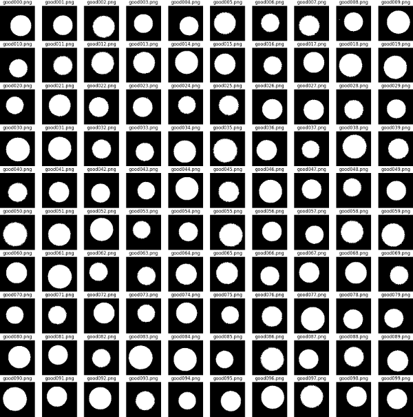
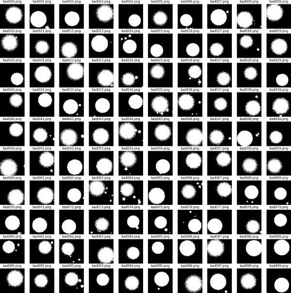
Using Numpy two datasets of 100x100 pixel black and white images are created. The first represents 'good' cases - these are circular with relatively distinct margins with no or only small amounts of splatter. In the second group of 'bad' cases - the welds are essentially circular but with one or more defects: the edge may be indistinct, the weld may be off centre and there may be a number of satellite splatter marks of significant size. The degree of accuracy in both sets is subject to random variation. Each image is represented by a square numpy array. We set up a coordinate system...
xx, yy = np.mgrid[0:IMAGESIZE, 0:IMAGESIZE]
and then draw a circle using the property that the circle radius is constant ie for a point (x,y) on the circle centred at zero (x**2)+(y**2)=(r**2)
pic = np.zeros((IMAGESIZE, IMAGESIZE), dtype=np.uint8)
pic = 255 * ((xx - cx)**2) + ((yy - cy)**2) <=(radius * noise)**2)
note (cx,cy) is the randomly varying circle centre
and 'noise' is a random variable controlling
the distinctness of the circle edge.
Below are examples of the images generated. We create a dataset of 1000 good images and 1000 bad images which will be used for training our machine vision model.
We use the Keras API of the Tensorflow python library (version 2.21). The Keras API presents a simplified interface for generating models which is more than adequate for our needs. The particular model we deploy is based on a layered neural network using 'convolutions'. In the general case, a neural network comprises layers of nodes, nodes in one layer connected to nodes in the subsequent layer. Input information flows through the nodes and iteratively weights, controlling how much influence each node has on its downstream connects, are adjusted so as to maximise the number of correct predictions by the model. Here we are interested in visual pattern detection and we can improve on the general case described above by representing the 2d structure of the data with a 2d structure in our layers and by only connecting nodes in one layer to close by nodes in the next layer. Preserving geographical structure in this way, maximises the chances of picking up local patterns such as edges and texture. Splitting up the network layer into small adjacent squares of neurons, the convolution (basically a matrix of the same small square size) applies its weights to the selected neurons and feeds this to the output. During the model training a number of different convolution filters are trained, allowing the model to focus on the different types of feature in the input picture. Note that the weights on the filter are constant as it scans over the input, meaning that it looks for the same feature at different locations. Feeding the output of one convolution layer as the input to another convolution means that the subsequent layer can be trained to look for collections of features found by the previous layer eg certain configurations or collections of edges. In this way, subsequent layers can pick up increasingly abstract concepts (e.g. a cat or a vehicle). Part of the art of constructing a network is deciding on the number of layers. Here we are looking at relatively simple geometric shapes - we use a model comprising three convolutional layers.
In order to help stabilise the model (so it converges on a solution rather than hunting or overfitting) we employ two tactics:
import tensorflow.keras as tfk
n_classes=2
model = tfk.models.Sequential(
[
tfk.Input(shape=(IMAGESIZE,IMAGESIZE,NUMCHANNELS)), #alert our model to the expected image size
tfk.layers.Rescaling(1./255), #convert our input image's 255s and 0s to 1s and 0s
tfk.layers.Conv2D(16, 3, padding='same', activation='relu'), #1st convolution layer
tfk.layers.MaxPooling2D(), #1st maxpooling layer
tfk.layers.Conv2D(32, 3, padding='same', activation='relu'),
tfk.layers.MaxPooling2D(),
tfk.layers.Conv2D(64, 3, padding='same', activation='relu'),
tfk.layers.MaxPooling2D(),
tfk.layers.Flatten(),
tfk.layers.Dense(128, activation='relu'),
tfk.layers.Dense(1, activation='sigmoid')
])
model.compile(optimiser='adam', loss='binary_crossentropy', metrics='[accuracy]')
Other points to note: the input images were saved as grayscale PNG ie a single channel where each pixel can vary from 0 (pure black) to 255 (pure white). When inputing the data we scale that to [0,1] without loss of data. Once we believe the stack of convolutions has extracted the necessary features (ie relative spatial position can be discarded) we convert that to a vector which is then input to a set of fully connected layers which has one final output representing the probability of class membership. To convert our continuously output to a binary 0 or 1 we apply a threshold 0.5. In order to compile the model ready for use we need to specify an optimiser and a loss function. The loss function measures the lack of fit of the model output with the ideal output. It is a quantity we want to minimise. Here we choose "binary cross-entropy", which is
(1/n)*sum[actual*log(prediction_prob) + (1-actual)*log(1-prediction_prob)]
Binary because our problem has two states, good or bad, modelled as 1 or 0 and "cross-entropy" because we are looking at the agreement or lack thereof between our actual data and our predictions. The optimiser controls how parameters in the model will be altered during training while searching for the best model. Many optimisers are based on 'gradient descent' i.e. changing parameters in the direction that gives the greatest reduction in the loss function. The "Adam" or Adaptive Moment Estimator is a safe choice. Based on gradient descent it uses refinements to improve the rate of convergence whilst maintaining stability. For any given observation, only one of the terms in the loss function will contribute, since either "actual" or "1-actual" will be zero. Note also that the loss function uses the prediction probabilities not binary classes ie larger errors have a greater effect than smaller errors. By taking logs we disproportionately penalise large errors - helping to nudge the model in the right direction during training.
We have an input dataset of 2000 images equally split between good and bad. We use 80% for training and hold back 20% for validation. The input data is divided into batches of 25. Small batches mean that the demands on system memory are controlled (at the expense of computation time). While small batches may also lead to less accurate estimates of the gradient used by the loss function (which is used in iteration to determine model fitness), paradoxically this may actually *improve* the model's generalisability by preventing it focussing too strongly on the peculiarities of the training data. The images are randomly shuffled so that the model does not learn or imply anything from the input order. Below are the results of training - five training runs or 'epochs' were used. (Experimentation showed that above 5 lead to some overfitting i.e. model accuracy on test data improving with no corresponding improvement when run on the validation data).
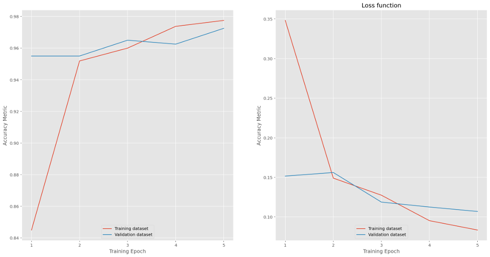 Evaluating performance of the model gives 98.2% accuracy and 0.068 loss for training data and 97% (0.11) for the validation data.
loss, accuracy = model.evaluate(train_ds)
loss, accuracy = model.evaluate(test_ds)
predictions model.predict(new_ds)
prediction_probs = ((predictions > 0.5).astype(int))
results = np.concatenate((predictions, predition_probs), axis = 1)
we see 992 correctly predicted good, 963 correctly predicted bad, 37 incorrectly predicted good and 8 incorrectly predicted bad i.e. an error rate of 45/2000 or 2.3%. Not bad for a first attempt. Reviewing the error cases, the majority seem to lie close to the boundary between the distribution of good cases and that of bad cases. These may in fact indicate a feature of the test data generator - the data follow random distributions meaning the two sets can overlap.
Back to other example analyses.