In the following we model the spread of a disease across a two dimensional space in discrete time.

Setting up the simulation

Rather than modelling the population as a homogenous entity, we assume a starting distribution over a geographical area and that transmission can only occur between proximal individuals. We model the geographical region using a 200x200 array. At a meeting of two individuals there is a 5% chance of transmission. We assume each individual meets 5 others per unit time interval. These meetings occur between individuals in the same or adjacent cell thus there is no transmission at a distance. If an individual is infected, they remain so for 14 days and then recover fully.

import numpy as np
import scipy.signal as spg
import scipy.stats as sps
p = 0.05 #probability of disease transmission at a single meeting
M = 5 #number of meetings per day for an individual
T = 100 #length of simulation run
gridsize = 200 #10x10 matrix representing geography
p_death = 0.0 #after 5 days infection either die or recover
recovery_time = 14

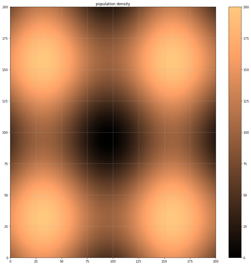
Let's now look at the population distribution. We'll use trigonometric functions to give us an undulating population spread, high points perhaps representing cities and low points the countryside. Our infected population will be modelled using a 3d array, 1 layer for each day the infection lasts.

population = (100+25*np.fromfunction(lambda x,y: np.sin(x/20)+np.sin(y/20), (gridsize,gridsize), dtype=float)).astype(int)
infected = np.zeros((gridsize,gridsize, recovery_time), dtype = float) #3d array - 1 layer for each day of infection
susceptible = population - infected.sum(axis=2)

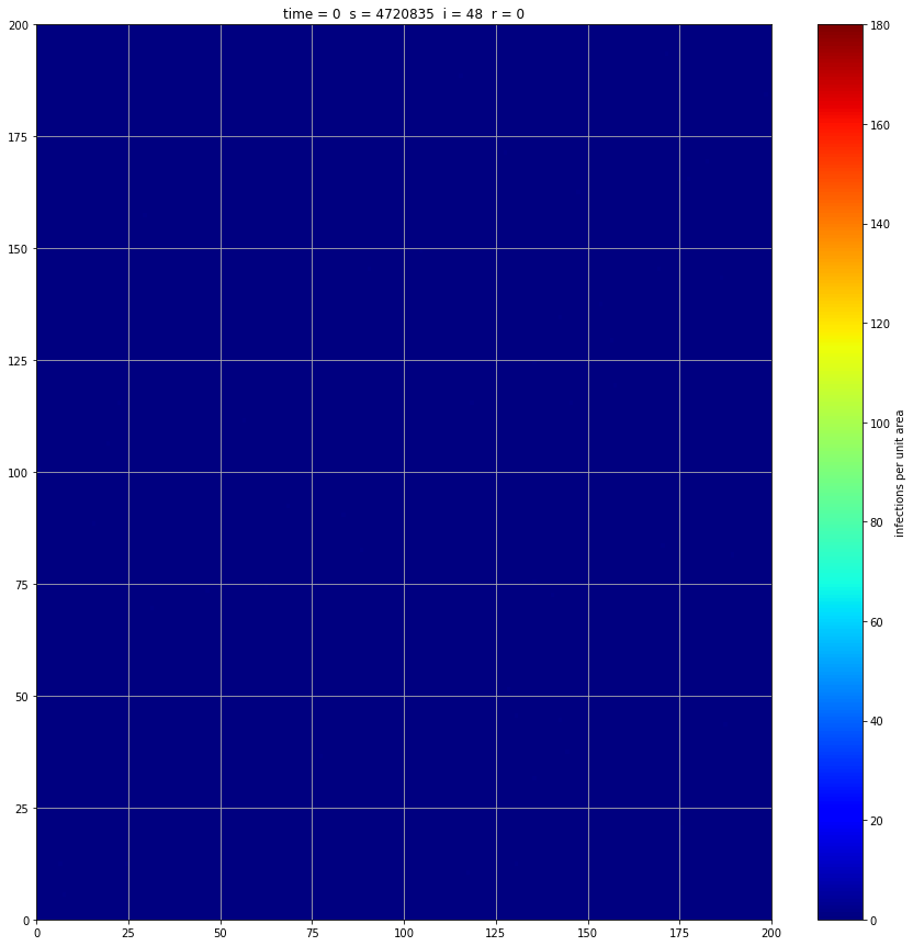
this is what the starting population looks like

import matplotlib.pyplot as plt
fig, ax = plt.subplots(1,1,figsize=(15,15)) ax.grid(True, linestyle='--', linewidth=0.5) plt.title('population density') plt.pcolormesh(population, cmap=plt.cm.copper, vmin=0, vmax=200) plt.colorbar()

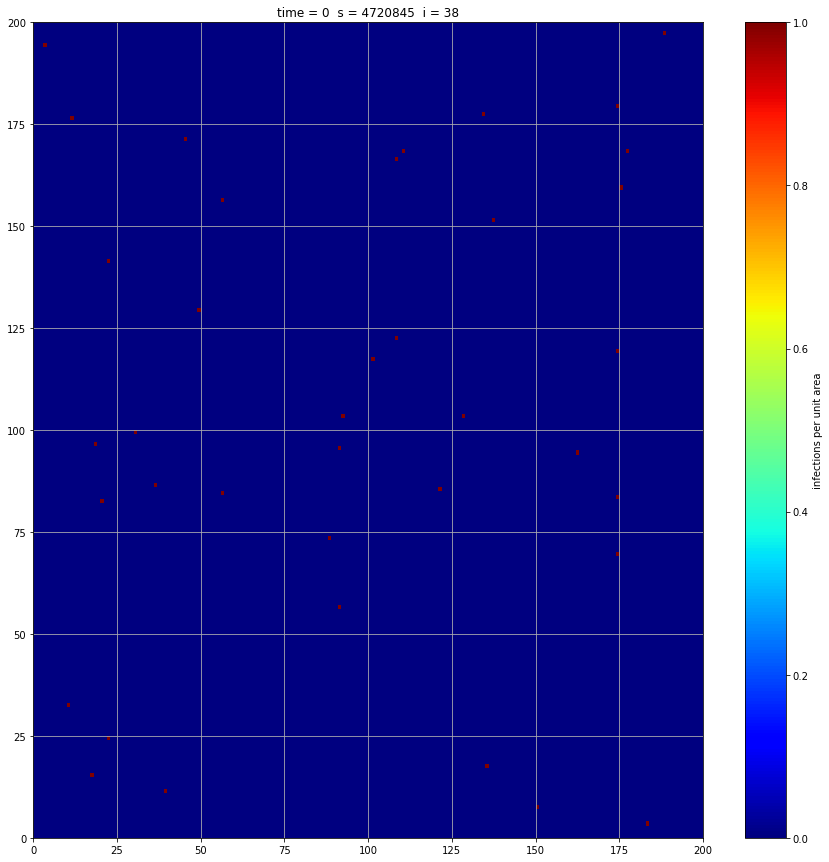
Now let's seed the population with a small number of initial infections. The rare infection events are modelled using the poisson distribution.

infected[:,:,0] = np.random.poisson(0.001,(gridsize,gridsize))

we'll use a 2d convolution to model the localised mixing of the population. Mixing of individuals occurs within a cell and between the cell and its eight adjacent cells.

weights = np.ones((3,3), dtype=float)

The Dynamics of Disease Spread

We will assume each individual has a fixed 'social capacity': in each time period they will have exactly M meetings. (Those in small communities will meet the same individuals multiple times.) Individuals stay within their community. We'll model meetings using the binomial distribution - implicitly we are assuming an individual can meet the same person multiple times. If the probability of transmission from an infected to an uninfected individual at a meeting is p, then the probability of transmission to an uninfected individual at a random meeting is p scaled by the proportion of the local population that is infected. We will inject some randomness into the simulation by sampling the number of new infections in a cell from the binomial distribution.

We're ready to start our main simulation loop. On each run we will for each cell (i) calculate the at risk population

results = np.zeros((T+1,2))
results[0] = susceptible.sum(), infected.sum()

for i in np.arange(T):

  #calculate local subpopulation relevant for each cell (cell plus immediate neighbours)
  local_total = spg.convolve2d(population - dead, weights, mode='same', boundary='fill', fillvalue=0)
  local_infected = spg.convolve2d(infected.sum(axis=2), weights, mode='same', boundary='fill', fillvalue=0)
 
  #calculate number of new infections
  p_infected = 1 - sps.binom.pmf(k=0, n=M, p=p*local_infected/local_total)
  new_infections = sps.binom.rvs(n=susceptible.astype(int), p=p_infected)
 
  #those on last day of infection all recover
  susceptible = susceptible + infected[:,:,recovery_time-1]
 
  #age existing infections by 1 day and insert new infection data
  infected = np.roll(infected, 1, axis=2)
  infected[:,:,0] = new_infections
  susceptible = susceptible - new_infections
 
  #store a summary of the position
  results[i+1] = susceptible.sum(), infected.sum()

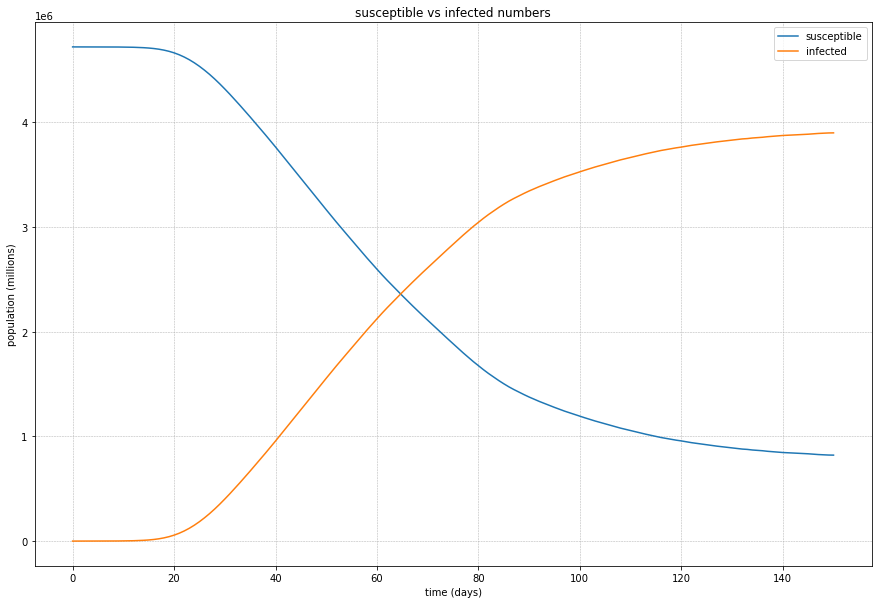
Looking at the summary results, we can see that the disease spreads through the population and stabilises at just over 80%.

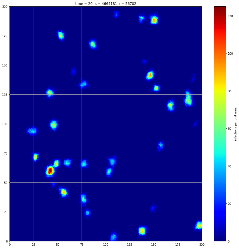
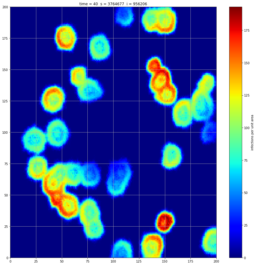
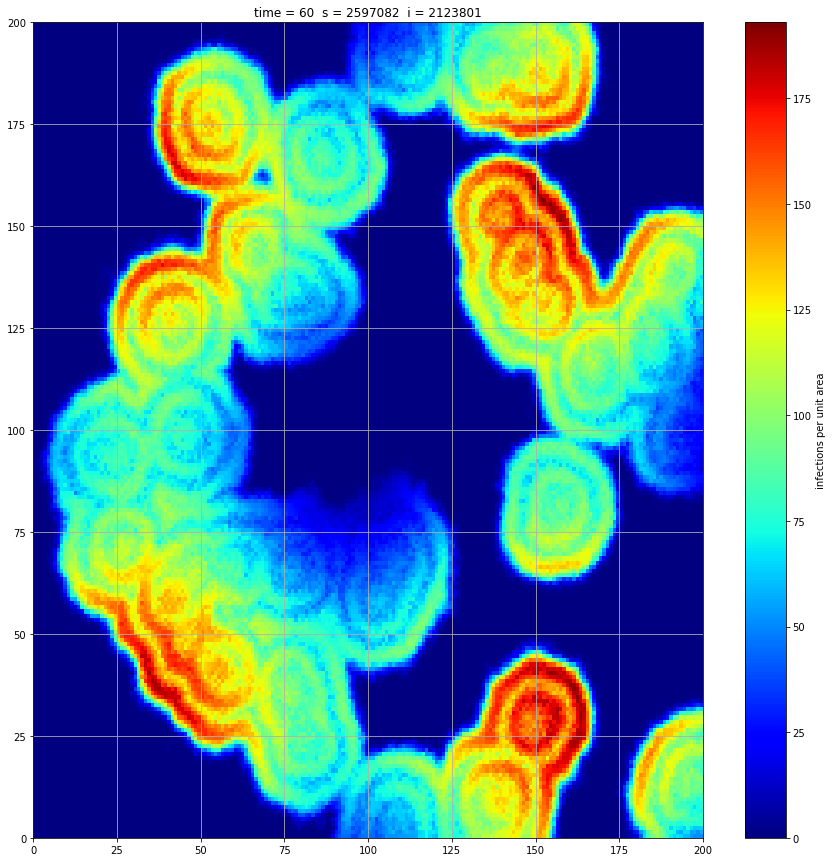
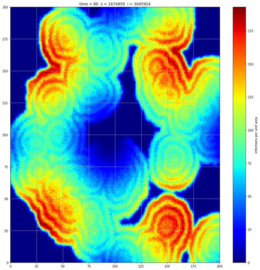
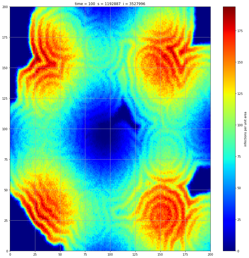
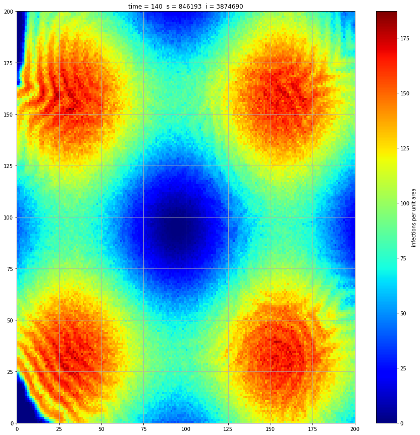
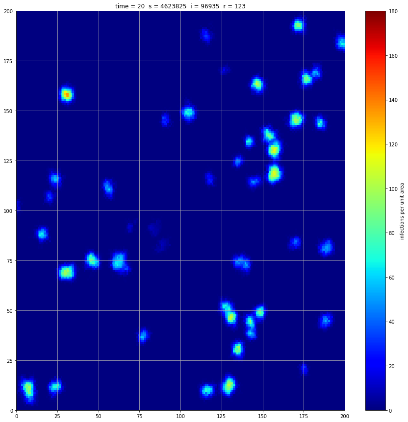
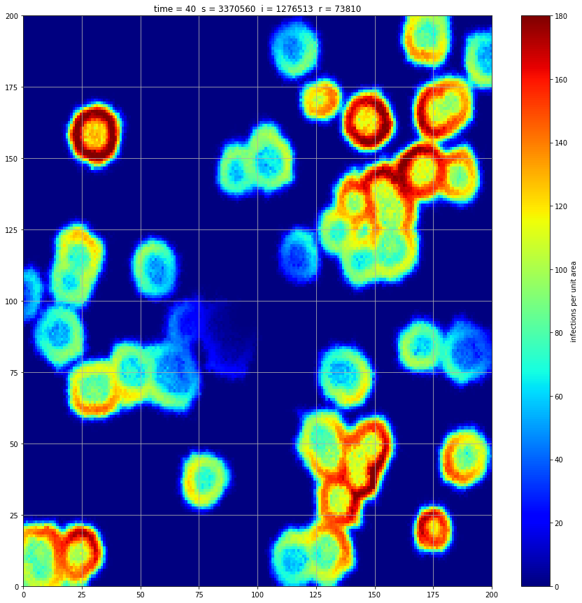
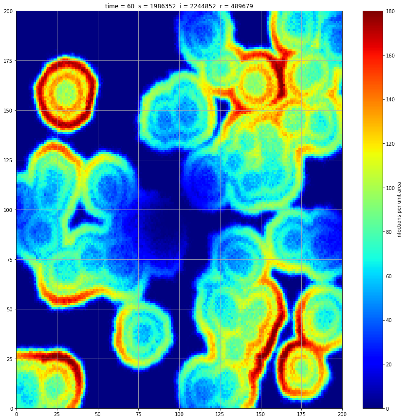
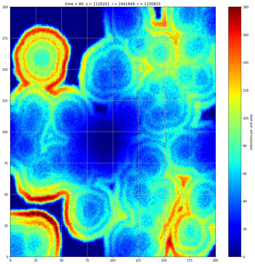
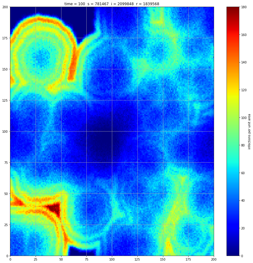
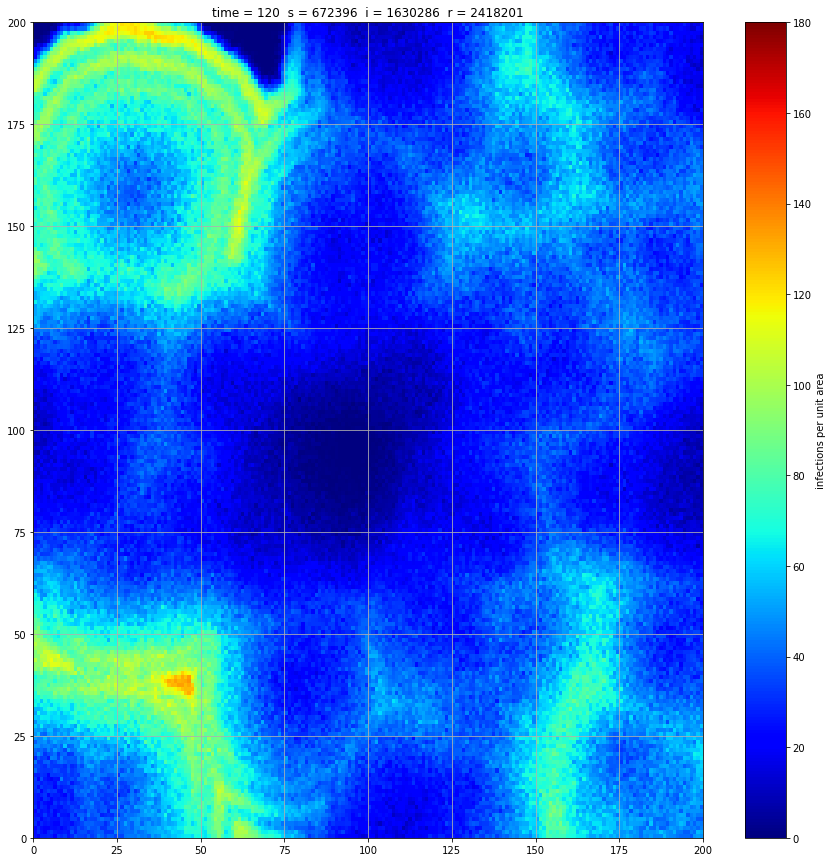
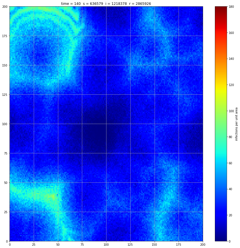
If we interrupt the simulation, we can see how the disease spreads geographically. Notice how the 14 day illness duration induces wavefronts in the spread. These wavefronts dissipate as the disease reaches a steady state where the number of new infections balances twith he number of recovers

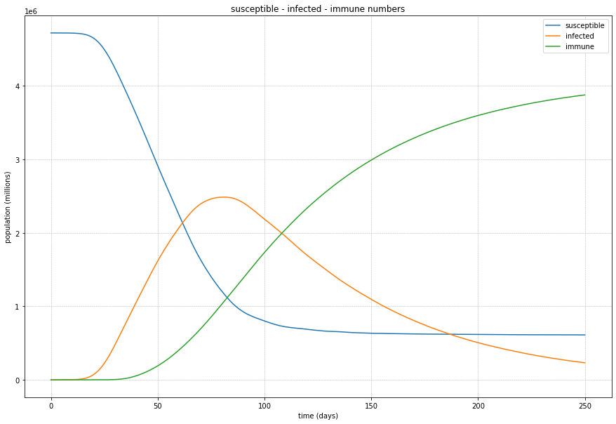
We can modify our simulation to introduce immunity. Let's say that at the end of a 14 day illness there is a 20% chance of developing immunity.

p_immune = 0.2
immune = np.zeros((gridsize,gridsize), dtype=float)

And our state transition code is augmented to account for the immune group

new_immune = np.floor(infected[:,:,recovery_time-1] * p_death + np.random.uniform(0,1,(gridsize,gridsize)))
immune = immune + new_immune
susceptible = susceptible + (infected[:,:,recovery_time-1] - new_immune)

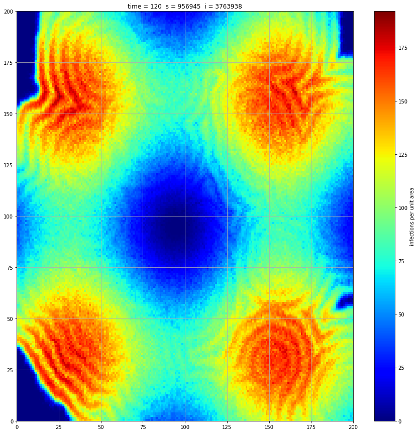
The result is a wave propagating through the population.

Back to other example analyses.