dS[t] = S*(mu*dt + sigma*dB[t])
where dS is the change in price S, and dB, the change in the process B which a sequence of normally distributed variables with mean zero. Mu is commonly known as the 'drift' and sigma as the volatility. Note, this implies that prices are a continuous process.
While it can be shown that market prices exhibit behaviours contracting the brownian motion hypothesis, the model nevertheless has a number of mathematical properties that make it a good starting point for simulation. Firstly, the roughness of brownian motion curve resembles the observed movements in market prices. Secondly, it implies prices are always positive. Thirdly, Brownian motion is the limit case of a random walk where the time step has been reduced to an infinitessimal value. In a random walk, the next value depends only on the current value, not on previous history. This matches the common hypothesis that markets efficiently price in all available information so that the next price movement depends only on the current price. Lastly, the foundation of brownian motion creates a tractable path for modelling option prices (see Black Scholes Merton model).
Going back to our differential equation - rearranging gives us...
(1/S)dS[t] = mu*dt + sigma*dB[t]
note (d/dx)(ln(x)) = 1/x so
(1/x)dx = d(ln(x))
substituting into the above...
d(ln(S[t])) = mu*dt + sigma*dB[t]
Next we use Ito's lemma for stochastic differentiation
(note we need a theory of differentiation for stochastic
processes because regular differentiation can not handle
functions that are infinitessimally rough like a Brownian motion curve)
to give us...
d(ln(S[t])) = (1/S[t])dS[t] + (1/(2S[t]**2))dS[t]dS[t]
substite this back in...
(1/S[t])dS[t] + (1/(2S[t]**2))dS[t]dS[t] = mu*dt + sigma*dB[t]
Going back to our original equation for a moment
dS[t] = S*(mu*dt + sigma*dB)
so
ds[t]*ds[t] = (S**2)((mu**2)(dt**2) + 2sigma*mu*dB*dt + (sigma**2)(dB**2) )
the first two terms can be ignored because dt tends to zero faster than dB
also dB**2 is order dt, so
ds[t]ds[t] = (s**2)(sigma**2)dt
(1/S)dS + (1/(2S**2)) (S**2)(sigma**2)dt = mu*dt + sigma*dB
(nb temporarily drop the [t] subscripts for brevity)
(1/S)dS + (1/2)(sigma**2)dt = mu*dt + sigma*dB
dS/S = mu*dt - ((1/2)sigma**2)*dt + sigma*dB
integrating...
INTG{1/S}dS = INTG{mu - ((1/2)sigma**2)*dt + sigma*dB}
INTG{1/x} = ln(x)
lnS[t] - lnS[0] = mu*t - (1/2)sigma**2)*t + sigma*(B[t] - B[0])
lnx - lny = ln(x/y)
S[t] = S[0]*exp((mu-0.5*sigma**2)t + sigma*B[t])
We can use this relationship to create a discrete time simulation. We'll create an array "s" to hold our simulated price series. Our simulation will last for "T" time (e.g. one year). Note the values of sigma and mu used are relative to this time period. We will break the simulation period into "steps" steps. Each step will be "dt" long.
T = 1 #duration of the simulation
steps = 260 #no. time-steps of the simulation
dt = T / steps #granularity of the simulation
sigma = 0.1 #price volatility
mu = 0.05 #price drift
s = np.zeros(T) #array to hold the simulated prices
s[0] = 100 #starting value for the price
B = np.random.normal(0,1, s.shape) #random variable determining brownian motion
for t in np.arange(1,steps):
s[t] = s[t-1] * np.exp( (mu-0.5*(sigma**2))*dt + sigma*(dt**0.5)*B[t])
Note, that vectorisation is always better than looping when using Numpy because it leverages the aspects of Numpy optimised for speedy processing. We can by induction show that the above is equivalent to
s = s0 * np.exp( np.cumsum((mu - 0.5*sigma**2)*dt + sigma*np.sqrt(dt)*B, axis=0))
which dispenses with the loop. The above simulates one asset price path. We can create multiple paths simultaneously via further vectorisation.
repeats = 1000
s = np.zeroes(T,repeats)
s[0,:] = 100
B = np.random.normal(0,1, s.shape) #this time creates a 2d array
s = s0 * np.exp( np.cumsum((mu - 0.5*sigma**2)*dt + sigma*np.sqrt(dt)*B, axis=0))
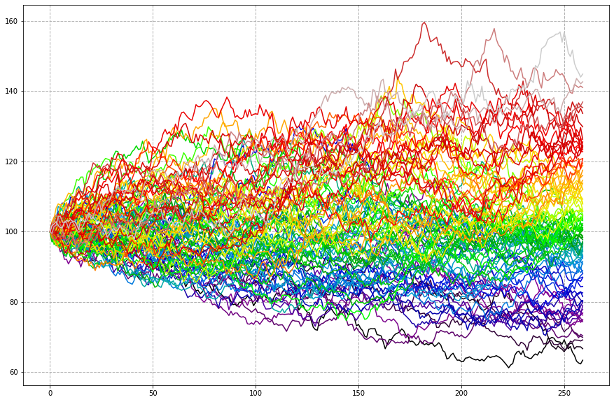
The plot below is the result of running the simulation 100 times (in parallel) for 260 days (roughly this many business days in a year).
S = S[:, S[repeats-1].argsort() ] #organise the series according to their end simulation value plt.subplots(1,1, figsize=(16,8)) ax = plt.subplot(1,1,1) ax.set_prop_cycle('color',list(plt.cm.nipy_spectral(np.linspace(0, 1, S.shape[1])))) ax.grid(True, linestyle='--', linewidth=1) plt.plot(S)
Note that
ln( s[t]/s[t-1]) = (mu-0.5*(sigma**2))*dt + sigma*(dt**0.5)*B[t]
i.e. we should find that our logged returns are normally distributed with mean (mu - 0.5sigma**2)dt and standard deviation sigma*(dt**0.5). This is indeed what binning and testing the data shows.
The main issue is that observed market prices just do not have the same distribution as brownian motion. The below compares the FTSE100 to brownian motion. The FTSE has fatter tails as evidenced by the kurtosis values. A second problem is that observations suggest volatility is not a constant but varies over time. Let's look at a sample of FTSE data...
import pandas as pd
import numpy as np
import matplotlib.pyplot as plt
import yfinance as yf
symbol='^FTSE'
tk = yf.Ticker(symbol)
price= tk.history(period="12mo").Close
fig, ax = plt.subplots(1,1,figsize=(15,5))
ax.grid(True, linestyle='--', linewidth=0.5)
ax.plot(price)
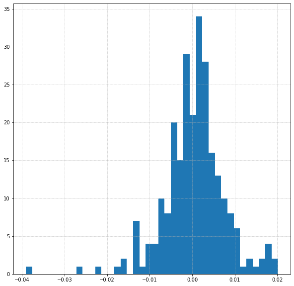
returns = price.pct_change().dropna()
logreturns = np.log(returns+1)
fig, ax = plt.subplots(1,1,figsize=(5,5))
ax.grid(True, linestyle='--', linewidth=0.5)
plt.hist(logreturns, bins=40)
How well do these data match up to the normal distribution - by eye its not a brilliant match. A few checks confirm this...
import scipy.stats as scs
scs.skew(logreturns), scs.kurtosis(logreturns)
Out[1]: (-0.7262008703980392, 3.9781186366758066)
scs.normaltest(logreturns)
Out[2]: NormaltestResult(statistic=48.75097016647868, pvalue=2.5933512019101312e-11)
scs.skewtest(logreturns, axis=0, nan_policy='omit', alternative='two-sided')
Out[3]: SkewtestResult(statistic=-4.38769776041585, pvalue=1.1455681652775608e-05)
scs.shapiro(logreturns)
Out[4]: ShapiroResult(statistic=0.946181058883667, pvalue=5.20902645462229e-08)
The test result p-values are very small and therefore highly significant. We reject the null hypothesis of normality in favour of the idea of non-normality (although see the separate post on the logic of hypothesis testing). The normaltest above directly looks at skew and kurtosis, the Shapiro-Wilks test looks at the overall shape of the distribution and the degree to which it differs from normal
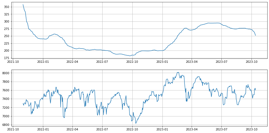
Pulling in a bit more historical data we can look at volatiltiy over time. We'll switch to Pandas because of the inbuilt time series functionality.
import pandas as pd
price_sd = price.rolling(260).std()
returns_sd_annual = np.sqrt(260)*returns_sd
fig, ax = plt.subplots(2,1,figsize=(16,8))
ax[0].grid(True)
ax[0].plot(price_sd['2021-11':'2023-10'])
ax[1].grid(True)
ax[1].plot(price['2021-11':'2023-10'])
Can we improve our simulation? Well, we can increase the kurtosis of the simulated data by including random 'jumps' up or down in the price series. This is the Merton Jump diffusion model. The frequency of jumps is modelled using the posson distribution with mean 'lambda' jumps per time period (we'll say 'lamb' in code because lambda is a reserved term). The size of the jumps is modelled by the normal distribution. The two changes compared to the brownian motion model are highlighted in bold: firstly an adjustment is needed to the price process drift and secondly there are the extra terms for the jump process.
B = np.random.standard_normal((steps, repeats))
jumpsize = np.random.normal(mu2, delta, (steps, repeats))
jumpadjust = lamb * (np.exp(mu2 + 0.5 * delta**2) - 1)
jumpfreq = np.random.poisson(lamb * dt, (steps, repeats))
for t in np.arange(1, steps):
S[t] = S[t-1] *
(
np.exp( (mu - 0.5*sigma**2 - jumpadjust)*dt + sigma * (dt**0.5) * B[t] )
+
(np.exp(jumpsize[t]) - 1) * jumpfreq[t]
)
We can also drop the constraint that variability is a constant. Instead our value of sigma might vary over time. We then need to decide the nature of that variation. Several models have been proposed. One is the Heston model where volatility is correlated with price. This model seems to work better for pricing options since it does produce a strike price vs implied volatility curve which more closely resembles those seen in markets (constant volatility as per the first model implies that volatility should not vary with price).
Back to other example analyses.